• What is the object detection problem?
• What is Intersection Over Union?
• How do you compare performance of multiple detectors?
• What are some of the detectors?
• What are sliding window detectors?
• What are some challenges with sliding window detectors?
• What is a Histogram of Gradients detector?
• What is Viola-Jones face detector?
• What are attentional cascades in neural networks?
• What is region-based convolutional neural network?
• Why from R-CNN to Fast R-CNN?
• What is Faster R-CNN?
• What is Region-based fully-convolutional network?
• What is You Only Look Once (YOLO)?
• How does 3D Object Detection work?

---

What is the object detection problem?

The goal of object detection is to detect the presence of object from certain set of classes and locate the exact position in the image. We can informally divide all objects into two big groups:

1. Things: are of certain size and shape like cars, people, etc. We can specify where they are using a bounding box.
2. Stuff: is more like a region of images which correspond to objects like grass or sky. It is easier to specify the location of a sky by marking the region in an image, not by a bounding box. To detect stuff, it is better to use semantic image segmentation methods.

To check whether the detection is correct, we compare the predicted bounding box with the ground truth bounding box. The metric is intersection over union.

\[\color{orange}{IoU = \frac{\text{Area of Overlap}}{\text{Area of Union}} \tag{1}}\]

---

What is Intersection over Union?

^{▴ Back to top}

The detector output is a set of detection proposals. Usually for each proposal the detector also gives a score as a measure of confidence in the detection. If IoU is larger than the threshold, then it is the true positive detection. If IoU is lower, then it’s false positive detection. If some ground truth object is not detected, then it is marked as misdetection or false negative.

On the whole dataset you can measure the precision and the recall of the detector. The precision is the ratio between the number of true detections and the number of all detections. The recall is the ratio of number of true detection to the number of objects annotated in the ground truth data.

---

How do you compare performance of multiple detectors?

^{▴ Back to top}

To compare two detectors correctly, you should compare their precision-recall curves. If one curve is generally higher than the other curve, then the first detector is better than the other. To measure the overall quality of the detector with one number, we compute average precision.

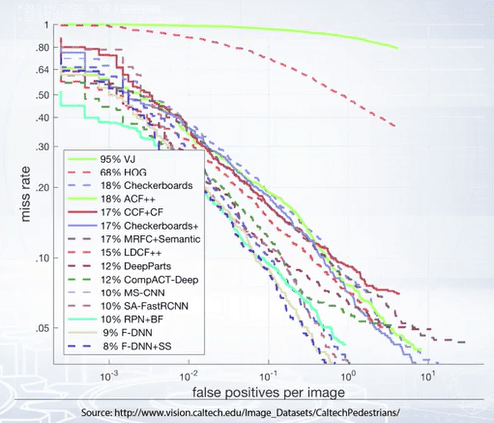
Another charting metric used is the plot of a miss rate with false detections per image. The curve is constructed similar to the precision-recall curve by varying the threshold on the detection score.

---

What are some of the detectors?

^{▴ Back to top}

1. Sliding Windows detector
2. Histogram of Gradients detector
3. Viola-Jones face detector
4. Attentional cascades

---

What are sliding window detectors?

^{▴ Back to top}

The main technique to reduce the problem of detection to image classification is sliding window. Consider a fixed size rectangular window, and you start sliding the window across your images, looking for the object you are trying to detect and asking the question “is Object?”. We mark all windows the classifier has said yes.

---

What are some challenges with sliding window detectors?

^{▴ Back to top}

Q1. How to handle various object sizes?

Solution: Use several windows of different sizes and scan image several times with different windows. Another technique is to downscale the images several times and create a multi scale pyramid. Then we can scan all scales in windows of same size.

Q2. How to handle various aspect ratio of objects?

Solution: Use windows of different aspect ratio. So, the number of images to be scanned equals to the product of number of scales and number of aspect ratio.

Q3. A lot of windows will have overlapped objects, so for each object you’ll get multiple positive responses, how to deal with this?

Solution: Score map of specific scale can contain multiple responses of various strength. To obtain final detection, we usually select points of local maxima, this non-maximal suppression is similar to how we detected edges in image gradient maps.

Q4. What if the object is partially overlapped with other objects?

Solution: In this case, the classifier should be really powerful to detect partially overlapped object, or we have to occupy only a small portion of the window.

---

What is a Histogram of Gradients detector?

^{▴ Back to top}

The idea of HOG detector is derived from using image edges as features. Image edges are robust features and sensitive to change in lighting. But edge maps, for example, Canny edge detector contain information only about modes of image gradients. Information about the gradient is lost in image maps.

Dalal and Triggs, in 2005 proposed to compute histograms of object gradients orientation and use them as feature of the image instead of edge maps. To do this:

1. Input Image: Take a sliding window of fixed size as an input.
2. Normalize gamma and color: Histogram normalization at the later stages made this step unnecessary.
3. Compute Gradients: Calculate image gradients as image convolution filter.
4. Weighted vote for spatial and orientation cells: Divide window into cells of eight by eight pixels. In each cell, calculate the histogram of gradient orientation. All orientations are divided into eight bins for example and vote for each pixel is weighted by gradient magnitude.
5. Neighboring cells are combined into blocks where each cell is included into several neighboring blocks. Histogram of all cells in the block are concatenated. Blocks can be rectangular or circular.
6. Contrast normalize over overlapping spatial blocks: Concatenated histograms in each block are then jointly normalized because each cell is included into cell blocks. After normalization, it produces several image features.
7. Collect HOG’s over detection window: All normalized histograms in all blocks are concatenated into final descriptor.
8. Linear SVM: Dalal and Triggs used linear support vector machine method for classification. Classifier gives a score and then we threshold it.

---

What is Viola-Jones face detector?

^{▴ Back to top}

Viola-Jones detector combines four key ideas:

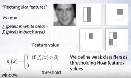
1. The simple Haar features: Haar features form a very large set of simple function. Each feature specify a set of rectangles in image window. We divide these rectangles into two groups, white and black. Feature value is calculated as difference between sum of pixels in white rectangles and sum of pixels in black rectangles. We define weak classifiers by thresholding Haar features. Such weak classifiers are sensitive to image gradients and other critical features in the image.

1. The use of integral images for fast feature computation: The integral image computes the value at each pixel, that is the sum of pixel values above and to the left of this pixel inclusive.

2. Boosting for feature selection: Boosting is an exhaustive greedy search. The training consists of several boosting round. For each round, we evaluate each rectangle filter on each example. We select best threshold for each weak classifier. We select the best combination of filter and threshold. We re-weight all examples. So, overall computational complexity of learning is proportional to the product of number of rounds, to the number of examples, to the number of features.

3. Attentional cascade for fast rejection of windows without faces: We start with simple classifiers which reject many of the negative windows while detecting almost all positive windows. The positive response from the first classifier triggers the evaluation of the second classifier, which is more complex and so on. A negative outcome at any point leads to immediate rejection of the window. Such attentional cascade allow us to apply slow classifiers only to a small subset of windows, which gives significant speedup to the algorithm.

Beyond Viola-Jones detector:

• Gradient-based features in form of integral channel features has been added to the detector.
• Faster ways for computation of such features in multi-scale mode has been proposed.
• Soft cascade and crosstalk cascades have been proposed to improve the detector speed.

---

What are attentional cascades in neural networks?

^{▴ Back to top}

CNN classifiers are very slow, so it is impractical to use them in sliding windows, but we can apply them as the last stage of attentional cascade. For example, we can use extension of Viola-Jones detector as proposal generator, and apply CNN only to the selected proposals. The next step is to replace all previous stages in attentional cascade to these neural networks.

In order to reach real-time performance, neural networks at the first stages should be very simple and fast. The number of stages can be reduced by using bounding box regression between stages. Bounding box regression take window as input and regress new bounding box position.

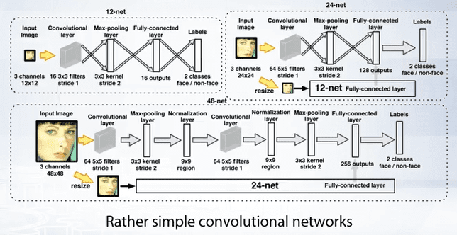
We can add separate neural networks after each stage of the Cascade to refine the bounding box of the proposal. In this particular algorithm, refinement of bounding box, is formulated as a classification problem. The classifier selects a transformation from a predefined set of transformations. Such classifiers are called calibration networks.

---

What is region-based convolutional neural network?

^{▴ Back to top}

In seminal work of Girshick et al, it was proposed to use external object proposal generator to obtain object proposals per image. Features are then extracted with convolutional neural network from these proposals and classified with SVM classifier. This method is called region-based convolution network or R-CNN.

In R-CNN, a selective search algorithm was used. Selective search is one of the generic object proposal generation methods. Such methods can provide high recall rate but very low precision. Thus they cannot be used as object detectors themselves, but they can be used as a first step in the detection pipeline.

Training Procedure:

1. A CNN is pre-trained on a larger dataset
2. The CNN is then fine tuned for object detection on limited object detection data set.
3. Linear classifier and bounding box regressors are trained on top of CNN features extracted from object proposals.

One very important advantage of R-CNN method is that it can use any convolutional neural network for feature extraction. You can improve the performance of R-CNN by using more advanced convolutional architecture. Thus switching from AlexNet to VGG leads to better mean average precision.

Problems with the R-CNN:

1. Redundant computations: All features are independently computed even for overlapped proposal regions.
2. Need to rescale object proposals to fixed resolution and aspect ratio.
3. Dependency on the external algorithm for hypothesis generation.
4. Complicated training procedure with high file system load.

---

Why from R-CNN to Fast R-CNN?

^{▴ Back to top}

Base CNN classifier used in R-CNN model due to fully convolutional layers requires an image with fixed resolution of 224 by 224 pixels as input. So, after objects proposals are extracted, they should be re-scaled to the fixed resolution, such a scaling changes object appearance and increased variability of images. But we can adapt any CNN classifier to various image resolutions by changing the last pooling layer, to the Spatial Pyramid Pooling or SPP layer.

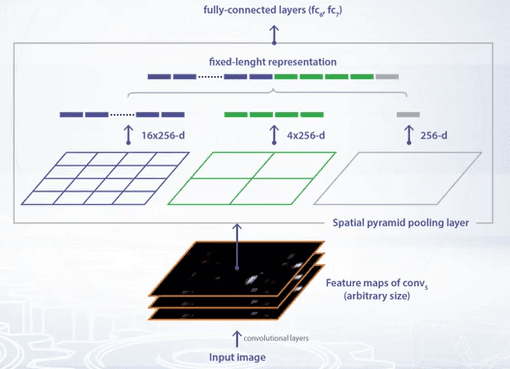
Spatial Pyramid is constructed on top of the region of interest. First level of the pyramid is a region of interest itself. On second level, the region is divided into four cells with two by two grid. On third level, region is divided into 16 cells on four by four grid. Average pooling is applied to each cell. So, if the last convolutional layer has 256 maps, then pooling in each cell produce one vector with length, 256. Feature vectors for all cells are concatenated, and then passed as input to the fully convolutional layer. Thus, we obtain fixed length feature representation for input images of various resolutions.

For each window, we apply Spatial Pyramid Pooling, and then compute fully convolutional layers for feature extraction. Compare this to computing convolutional features for each of the 2,000 object proposal. This leads to a dramatic increase in processing speed. In this Fast R-CNN paper, Girshick has proposed to use the Region of Interest Pooling layer, or ROI layer. It’s a simplified depiction of SPP layer, there is only one pyramid layer.

In addition to Region of Interest Pooling, two more modifications have been introduced.

1. Softmax classifier is used instead of SVM classifier.
2. Multi-task training is used to train classifier and bounding box regressor simultaneously.

Training Procedure:

1. The input image and set of object proposals are supplied to the neural network.
2. The neural network produces a convolutional feature map. From convolutional feature map, feature vectors are extracted using Region of Interest Pooling layer.
3. Then, the feature vectors are fit into a sequence of fully convolutional layers. The output of fully convolutional layers are branched into K-way softmax, and K by four real valued bounding box coordinates output.

Fast R-CNN can be trained to this multi-task loss:

\[\color{orange}{L(p,u,t^u,v) = L_{cls}(p,u) + \lambda[u \geq 1]L_{loc}(t^u, v) \tag{2}}\]

This multi-task loss is the rate of sum of classification loss:

\[\color{orange}{L_{cls}(p,u) = -logp_u \tag{3}}\]

And bounding box regression loss:

\[\color{orange}{L_{loc}(t^u,v) = \sum_{i \in (x,y,w,h)}smooth_{L_1} (t_i^u - v_i) \tag{4}}\]

where $t^u = (t_x^u, t_y^u, t_w^u, t_h^u)$

For the true class U, log loss is used. The smooth L1 loss is used for the bounding box regression.

Problems with the Fast R-CNN:

1. For the Fast R-CNN, when we use different images in one batch, the computations are expensive for each window, because in Fast R-CNN convolutional features are extracted from the whole image, the receptive field for the Region of Interest Pooling is very large. In worst case, it can be entire image. So for each example, we need to compute convolutional features for the entire image.
2. The one last weak point of R-CNN, is the dependency on external hypothesis generation method.

---

What is Faster R-CNN?

^{▴ Back to top}

Faster R-CNN is Fast R-CNN plus Region Proposal Network. In Faster R-CNN, the last main problem of R-CNN approach is solved. The dependency from the external hypothesis generation method is removed. Objects are detected in a single pass with a single neural network.

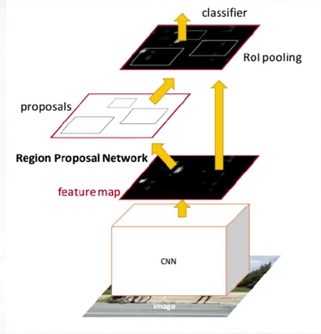
RPN is a simple fully convolutional network which is trained to its multitask loss, similar to Fast R-CNN, and serves as a proposal generator.

The Region Proposal Network is a small network that is slid over convolutional feature map.

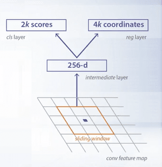
This small network takes its input and then by N spatial window usually N equals 3. RPN simultaneously classify corresponding region as object or non object in the regress bounding box location.

Position of the sliding window provides localization information with reference to the image. Box regression provides finer localization with the reference to this sliding window itself. At each sliding window position a set of object proposals is defined. Each proposal has different size and aspect ratio. Such proposals are called anchors.

Anchors improve handling of objects of different size and aspect ratio. Essentially anchors is a variant of sliding window with different sizes and aspect ratio.

Proposal Network anchor is marked as positive example if intersection over union is larger than 0.7, or it reaches maximum for all anchors for this particular ground truth example. Anchor is marked as negative sample if IoU is lower than 0.3.

Faster R-CNN can be trained end to end as one network with four losses. RPN classification loss, RPN regression loss, Fast R-CNN classification loss over classes, Fast R-CNN regression loss to regress the proposal bounding box to the ground truth bounding box.

Problem with the Faster R-CNN:

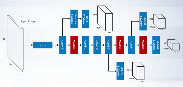
1. However, despite the anchor boxes, it can be difficult for RPN to handle objects of very different scales. RPN has fixed receptive field. So small objects can occupy a very small portion of receptive field or if objects are very large then the receptive field will contain only a part of the object.

We can solve this problem by training a set of RPN for various scales. Each RPN will take different convolutional layer or set of layers as input so the receptive field will be of different size. This will significantly improve detection of small and large objects so one Faster-RCN model can detect simultaneously objects from small to large sizes.

---

What is Region-based fully-convolutional network?

^{▴ Back to top}

Region-Based Fully Convolutional Network is a modification of faster R-CNN, but it can be regarded as one of the meta-architecture of modern CNN-based object detectors.

The key idea for the regional-based fully convolutional network is to pre-compute box classifier features once for the whole image. Then crops are taken from the last layer of features prior to prediction. In this model, fully connected layers are replaced with convolutional layers.

To make strong classifier, a committee of region-based position-sensitive classifiers is built. For each class, k by k, position sensitive score on maps are generated by fully convolutional network. In a region of interest pooling, k by k grid is used. But for pooling in each cell, only one of the maps is used. In this light, used maps are visualized with different colors. Each positional sensitive feature maps predicts high confidence only if object is located at predefined position relative to the region of inter-cell.

Full regional fully convolutional network model contains RPN and region-based classifiers. All components of the model can be jointly trained to multitask loss.

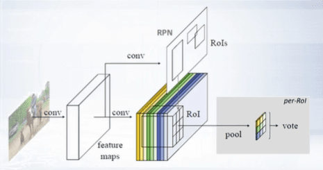
The main advantage of this meta-architecture compared to the faster R-CNN model is that it’s computational speed is weakly dependent on the number of proposals, which can significantly increase the number of the proposal whereas some RPN network show only moderate increase in computational time for the whole detector.

---

What is You Only Look Once (YOLO)?

^{▴ Back to top}

The rationale behind calling the system YOLO is that rather than pass in multiple subimages of potential objects, you only pass in the whole image to the deep learning system once. Then, you would get all the bounding boxes as well as the object category classifications in one go.

The way YOLO works is by subdividing the image into an NxN grid, or more specifically in the original paper a 7x7 grid. Each grid cell, also known as an anchor, represents a classifier which is responsible for generating K bounding boxes around potential objects whose ground truth center falls within that grid cell (K is 2 in the paper) and classifying it as the correct object.

For more dense object detection, a user could set K or N to a higher number based on their needs. However, with the current configuration, we have a system that is able to output a large number of bounding boxes around objects as well as classify them into one of various object categories, based on the spatial layout of the image.

This is done in a single pass through the image at inference time. Thus, the joint detection and classification leads to better optimization of the learning objective (the loss function) as well as real-time performance.

---

How does 3D Object Detection work?

^{▴ Back to top}

LiDAR and Depth Sensors gives 3D information of the world around it, which can’t be directly captured by passive 2D camera setup. The techniques we discussed are trying to detect the objects in the raw point clouds without any texture information (just with the representation of the position (x,y,z)).

There are few reasons why it is a good idea to look into 3D detection directly on point cloud:

1. There is no single compact sensor like we have kinect sensor (indoors) for self driving cars (because of range issue).
2. Because of the above reason we had to use two separate sensors, camera and LiDAR. When the car is moving and lidar is rotating, the point cloud that is registered for one spin is distorted because of car motion.
3. When you want to project this LiDAR depth information on to camera, it needs to exactly synchronize with the camera (timestamp should be almost same, there should be a common clock for both the sensors).
4. Then it can be projected on to the camera after correcting the motion distortion in the point cloud using other sensors like GPS/IMU.

A typical point cloud consists of four different values (x, y, z and r) corresponding to the x, y and z co-ordinates of the point of which the light ray was reflected off and r being the reflectance.

---

️⭐️ Coming up Next: Computer Vision: Object Tracking

If you need more explanations, have any doubts or questions, you can comment below or reach out to me personally via Facebook or LinkedIn, I would love to hear from you 🙂.

🔔 Subscribe 🔔 so you don’t miss any of my future posts!